This page explains the statistical methodologies underlying the analysis presented in “Environmental justice implications of CSO outfall distribution”.

Bootstrapping for visualization

We visualize the trend in CSO discharge volume by dividing the watersheds into four equal-sized bins according to each of the three EJ criteria defined by the state of Massachusetts and using bootstrap resampling to estimate the uncertainty in the population-weighted mean discharge volume estimate in each bin.

Regression modeling for dependence measurement

We measure the dependence of the CSO discharge outcome on EJ indicators using a Bayesian population-weighted logarithmic regression model as follows,

$$y \sim \textrm{N}(\theta, \sigma/\sqrt{p})$$

$$\theta = \alpha ~ x^{\beta}$$

where y (dependent variable) is the annual volume of CSO discharge in gallons, x (independent variable) is the watershed-level EJ population indicator (linguistic isolation, income, or minority population) as a fraction, and p is the total population of Census blocks in the watershed. N is the normal distribution (defined such that the second argument is the standard deviation and not the variance). The parameter β (the parameter whose inference this analysis is focused on) represents the univariate dependence of CSO discharge on each EJ indicator, α represents the offset (zero-point) between the dependent and independent variable, and σ represents the noise or “error” in the dependent variable data.

We assign weakly informative priors (see e.g. Sanders & Lei 2018) to the parameters of this model as follows,

$$\sigma \sim \textrm{N}(0, 4)$$

$$\alpha \sim \textrm{N}(0, 10~\textrm{sd}(y))$$

$$\beta \sim \textrm{N}(0, 4)$$

where sd is the standard deviation function.

The model is fit using the pystan probabilistic programming language and inference tool using Hamiltonian Monte Carlo.
The exact Stan code for the model described above is available in the AMEND repository.

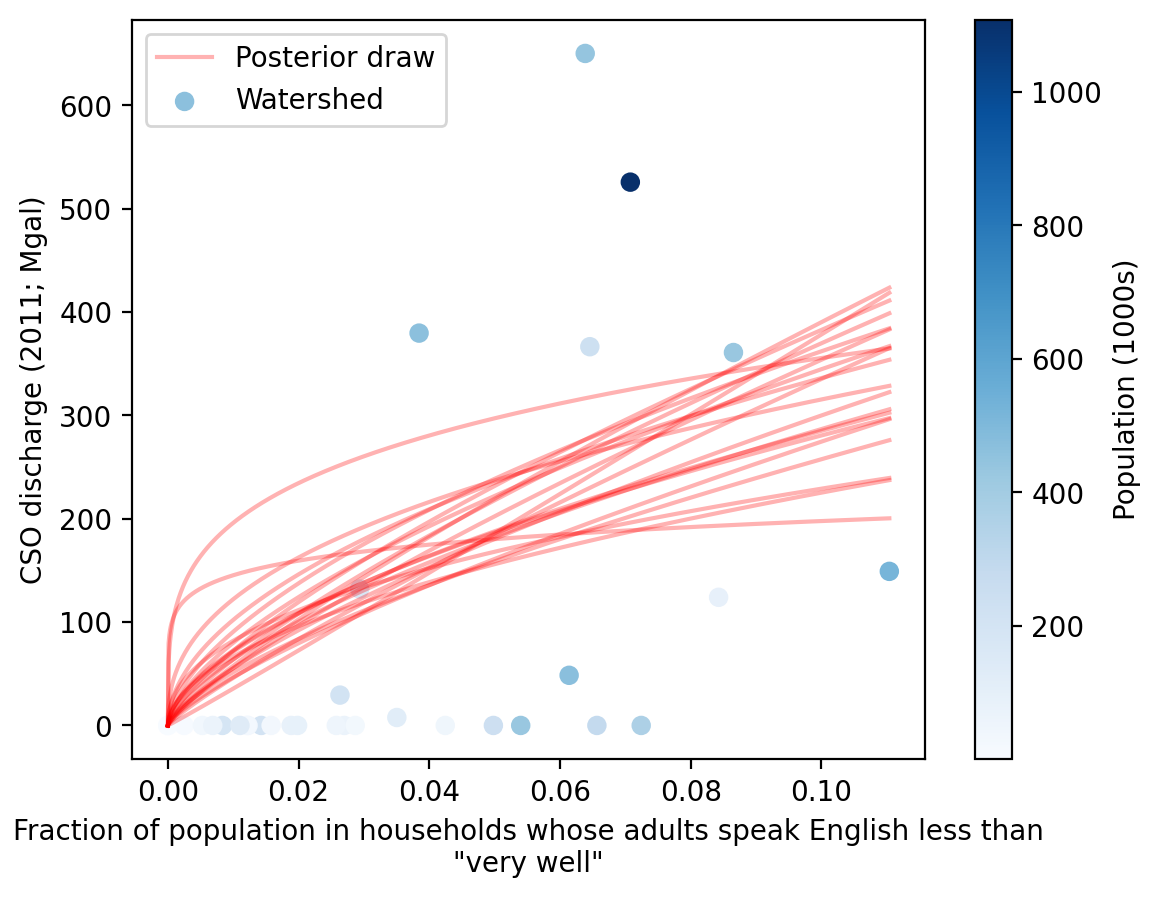
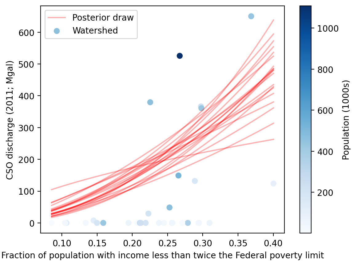
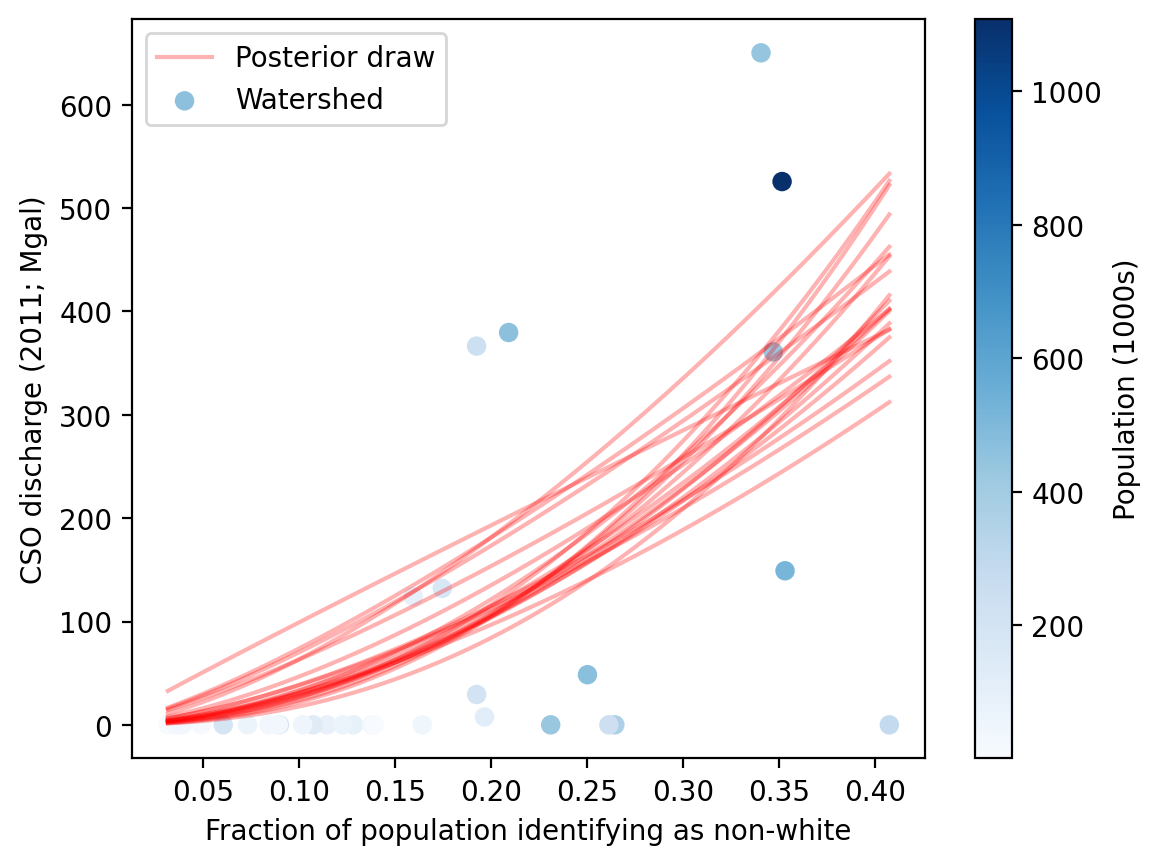
The plots below illustrate the functional form of the fitted model for each EJ indicator.
A sample of random draws from the Markov Chain posterior are shown in red.
The actual watershed data points are shown in blue, colored according to the watershed population used to weight the model fit.

The plots below show the posterior probability distribution of the dependence measurement β for each EH indicator, transformed as \(2^\beta\) to represent the growth of the dependent variable corresponding to a 2x increase in the independent variable.

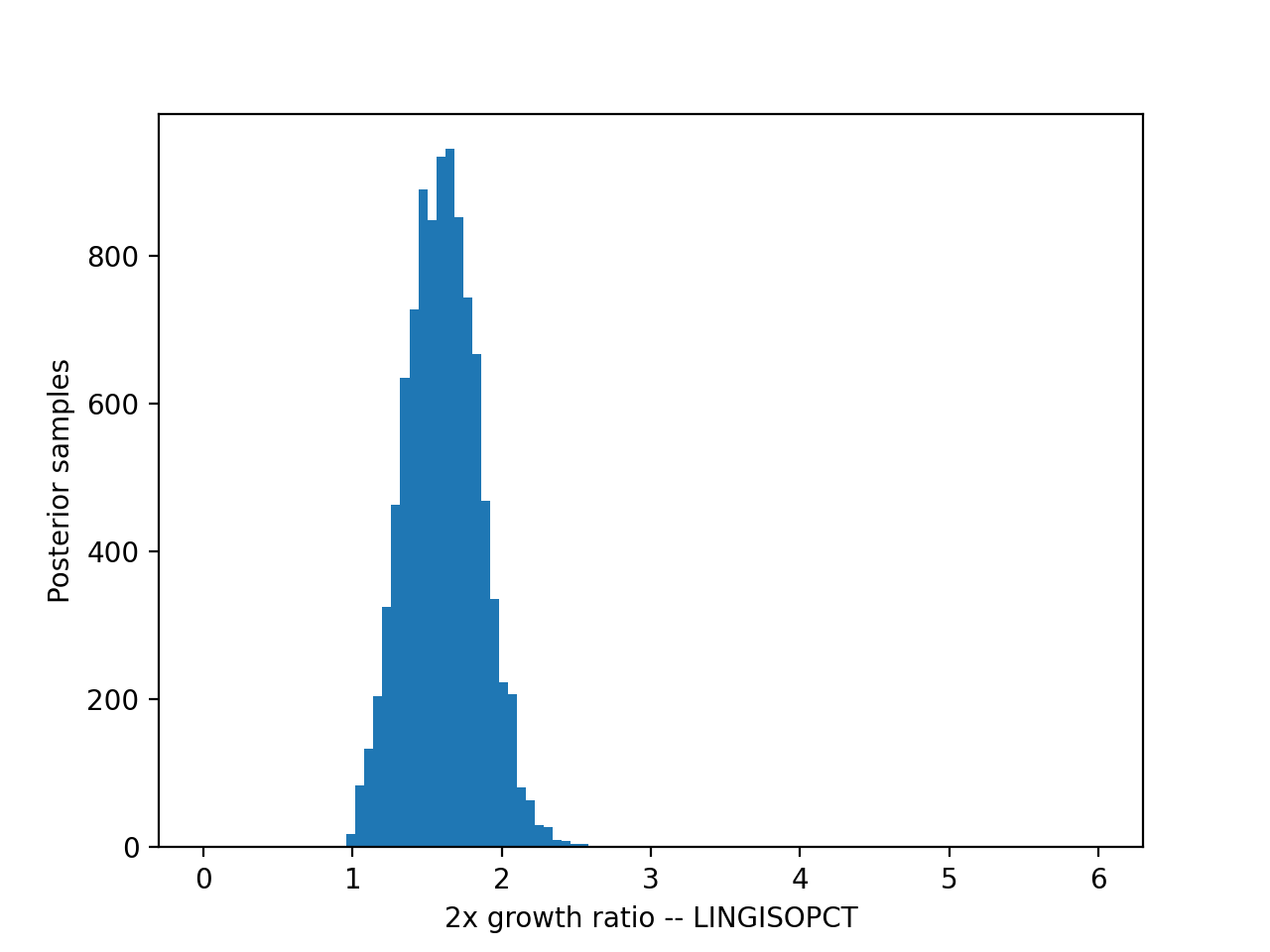
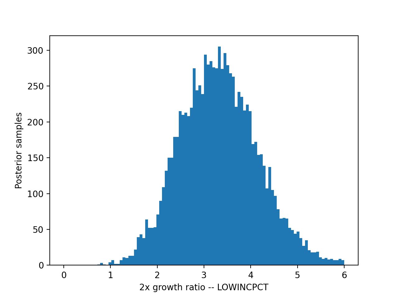
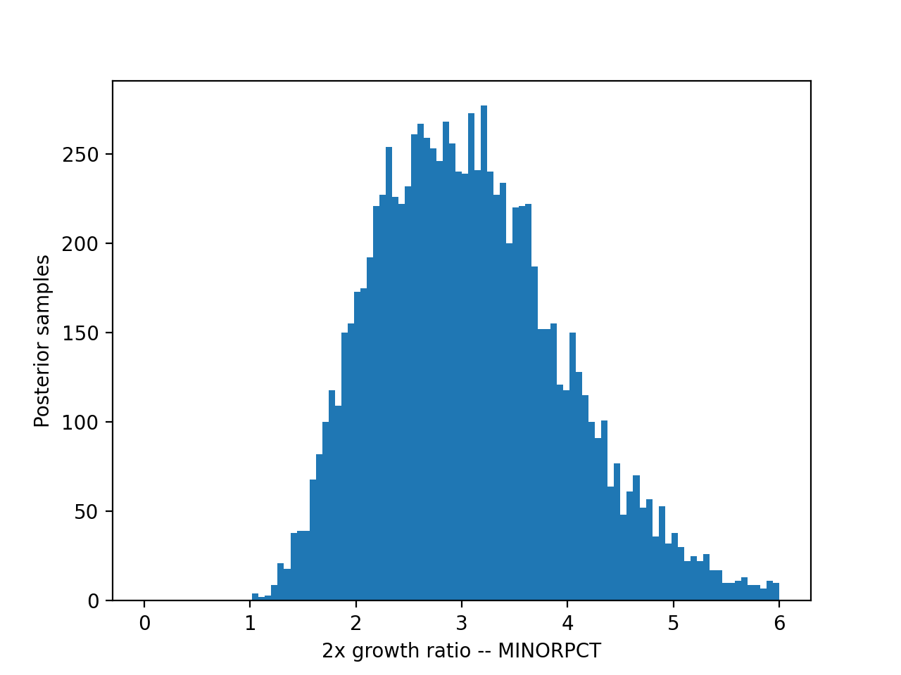
The 90th percentile posterior (confidence) interval of these distributions are quoted in the analysis page.